The big idea
Close to the point of contact, a curve and its tangent line are almost the same. That makes the tangent a cheap way to approximate a function. The Mean Value Theorem says that somewhere on an interval the instantaneous rate must equal the average rate.
Key ideas
- Tangent line at x = a: y = f(a) + f′(a)(x − a). The normal line has slope −1/f′(a).
- Linear approximation: f(x) ≈ f(a) + f′(a)(x − a) for x near a.
- The approximation is an underestimate where the curve is concave up and an overestimate where it is concave down.
- MVT: if f is continuous on [a, b] and differentiable on (a, b), then f′(c) equals the average rate of change for some c in (a, b).
- Rolle's theorem is the special case f(a) = f(b), which guarantees a point with f′(c) = 0.
Equations
| L(x) = f(a) + f′(a)(x − a) | linearisation at a |
| f′(c) = [f(b) − f(a)]/(b − a) | Mean Value Theorem |
| mnormal = −1/mtangent | perpendicular slopes |
| f(a) = f(b) ⇒ f′(c) = 0 | Rolle's theorem |
Worked questions: easy, medium, hard
Three questions that climb in difficulty, each solved one step at a time. Try each one before you read the steps.
Find the tangent line to y = x3 − 2x at x = 2.
- Point: y = 8 − 4 = 4, so (2, 4).
- Slope: y′ = 3x2 − 2, which is 10 at x = 2.
- Line: y − 4 = 10(x − 2), that is y = 10x − 16.
Use a linear approximation to estimate √26.
- Choose f(x) = √x and the nearby easy point a = 25.
- f(25) = 5 and f′(x) = 1/(2√x), so f′(25) = 1/10.
- L(26) = 5 + (1/10)(26 − 25) = 5.1.
- The curve √x is concave down, so 5.1 is a slight overestimate (the true value is 5.099).
Find the value of c guaranteed by the Mean Value Theorem for f(x) = x3 − 3x on [0, 2].
- f is a polynomial, so it is continuous and differentiable everywhere. The MVT applies.
- Average rate: [f(2) − f(0)]/(2 − 0) = (2 − 0)/2 = 1.
- Set f′(c) = 3c2 − 3 = 1, so c2 = 4/3.
- c = ±1.155, and only c = 2/√3 ≈ 1.155 lies in (0, 2).
Common mistakes
- Using the MVT without checking continuity and differentiability.
- Giving a value of c that lies outside the open interval.
- Using the slope formula with the wrong point when writing a tangent line.
Now you try: easy to hard
Six more questions, two at each level. These are the questions on the worksheet; each solution opens when you are ready.
Easy 1. Find the normal line to y = x2 at (1, 1).
Show the step-by-step solution
Tangent slope: 2x = 2. Normal slope: −1/2. Line: y − 1 = −(1/2)(x − 1).
Easy 2. Where is the tangent to y = x2 − 6x + 5 horizontal?
Show the step-by-step solution
y′ = 2x − 6 = 0 at x = 3. y = 9 − 18 + 5 = −4. The point is (3, −4).
Medium 3. Linearise f(x) = ln x at x = 1 and estimate ln 1.1.
Show the step-by-step solution
f(1) = 0, f′(1) = 1, so L(x) = x − 1. ln 1.1 ≈ 0.1 (true value 0.0953).
Medium 4. Verify Rolle's theorem for f(x) = x2 − 4x on [0, 4] and find c.
Show the step-by-step solution
f(0) = 0 and f(4) = 0, and f is a polynomial, so the theorem applies. f′(c) = 2c − 4 = 0 gives c = 2.
Hard 5. Find the c guaranteed by the MVT for f(x) = √x on [1, 9].
Show the step-by-step solution
Average rate: (3 − 1)/(9 − 1) = 1/4. f′(c) = 1/(2√c) = 1/4 gives √c = 2, so c = 4.
Hard 6. Use a linear approximation to estimate the cube root of 8.06.
Show the step-by-step solution
f(x) = x1/3, a = 8. f(8) = 2, f′(x) = (1/3)x−2/3, f′(8) = 1/12. L(8.06) = 2 + 0.06/12 = 2.005.
6 questions to print or save, with full step-by-step answers at the end.
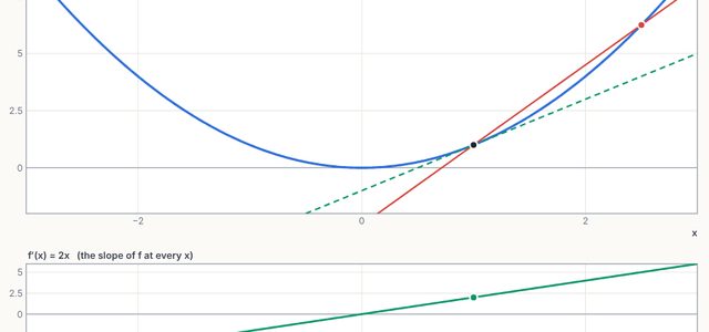
Open the Derivative Explorer simulation and test every idea on this page yourself.
Open the simulation →